Basic Hardware Rendering

Dedicated gaming hardware has a struggled history, especially in the PC space where games relied on pure software rendering until the mid 90s. Nowadays though low cost computers dedicate a third or more of their CPU’s transistor budget to graphics while higher end systems ship with dedicated graphics chips. All of those transistors are primarily optimized to make games look nicer. It’s a favorable situation for game programmers. However the forefront of technology is an adventurous environment. GPU (graphical processing unit) development tools are not yet as mature as CPU focused development tools and incompatibilities and driver bugs can eat up development time faster than a piranha poodle eats up his lunch.

Today’s GPUs are massively parallel chips that can do hundreds of calculations in parallel. This distinguishes them clearly from CPUs which are primarily optimized to run sequential code as fast as possible and only adopted multicore architectures because progress in further accelerating sequential code stagnates. Additionally GPUs contain some fixed function hardware, most importantly for texture sampling and triangle rasterization.

Triangles

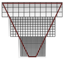
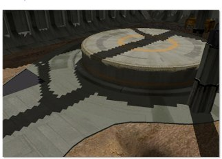
Triangles as created by GPUs look jaggy with default settings.

This happens when only one point per pixel is sampled to render a triangle. Low sampling frequencies also lead aliasing artifacts aka a loss of information – when a triangle is about as thin or thinner as the distance between two samples it can disappear depending on its exact position. Calculating more than one sample per pixel is called Supersample Antialiasing in gaming jargon. It’s an effective and simple but also resource hungry technique. Modern graphics chips support an alternative technique called Multisample Antialiasing which only calculates additional samples at triangle edges. Efficiency then depends highly on typical triangle sizes.

Anti-Aliasing generally also helps smoothing jaggy triangle edges but recently more and more games employ algorithms which only help smoothing triangle edges but do not fight any actual form of aliasing. After the image is rendered edge detection filters are applied to smooth hard edges. Those algorithms are usually called anti-aliasing, too, although that is not technically correct. Other more current algorithms try to remap previously calculated frames into the current frame, then blend them together in a procedure called temporal anti-aliasing. This works best with slow moving cameras because remapping a 2D frame to a new 3D position is not a perfectly reliable process. Temporal anti-aliasing can however remove actual aliasing.

Older graphics chips could also directly rasterize properly anti-aliased triangles. But this process, called Edge Anti-Aliasing, produces semi-transparent pixel values and accordingly triangles would have to be sorted for correct visuals and the process does not work for overlapping triangles.

Textures

Textures are basically images. Sometimes though textures consist of multiple images. Some graphics chips or graphics apis (like WebGL) prefer or only support texture widths and heights of 2^n, but it’s always possible to put an image that does not fit this constraint in a larger texture and modify texture coordinates accordingly.

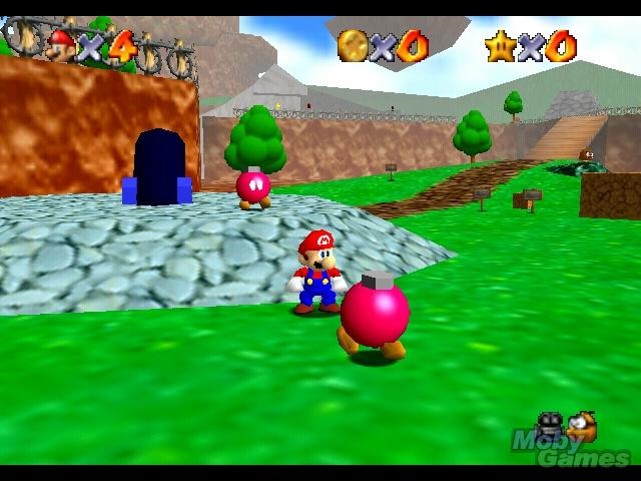
GPUs can fetch texture data by either just getting the pixel nearest to the supplied texture coordinate or by interpolating the four surrounding pixels, which is called point and bilinear filtering, respectively. Most 3D games always use bilinear filtering which leads to the typical smeary textures which can be found in almost any 3D game.

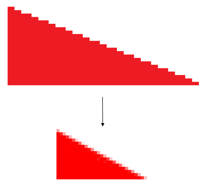
Bilinear filtering can be very useful when textures are scaled up, but it does not help much when textures are scaled down. When a large texture is drawn across a very small triangle ideally for every drawn pixel a large amount of texture pixels (called texels) would have to be interpolated – in the extreme case when a complete texture is mapped to a single pixel that pixel should have the mean value of all texels. Sampling textures like that however is not feasible in realtime rendering. Instead scaled down textures are precalculated, typically at (width/2, height/2), (width/4, height/4), and so on. Those are called mip maps and graphics apis can treat a complete mip map chain like as a single texture. When rendered the best fitting mip map level is chosen for texel sampling. To avoid artifacts at mip level boundaries, which are very clearly visible during movement along prespectively stretched walls, mip maps can be sampled using trilinear filtering, sampling and interpolating from two mip levels for every pixel. Trilinear filtering though also doesn’t work perfectly with perspective, because perspective projections tend to scale to different sizes in x and y directions, making it impossible to choose optimal mip levels. This results in images which are either smeary (aka scaled up from a smaller mip level) or grainy (suboptimally scaled down from a bigger mip level).

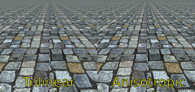
Graphic chips support an anisotropic texture filtering mode to avoid these artifacts, which incorporates more samples when textures are stretched unevenly in x and y. How good anisotropic filtering actually works is usually effected by user level options in the graphics driver menus, at least on Windows.

Depth Buffer

The depth buffer algorithm is implemented as part of the rasterizer and thus can only be configured using the graphics api. Typically it can be switched on and off and reject either higher or lower z values compared to previous z values.

Alpha Blending

Transparency or alpha blending as it is usually called is a stressful procedure for any graphics chip. Incorporating previous color values stresses the memory interface and makes parallelization of calculations more difficult, because earlier triangle calculations must be completely finished before pixels can be blended. For those reasons alpha blending is still not a programmable process on most chips (modern chips which use deferred rendering, like the PowerVR chips used in iOS devices are an exception). Instead alpha blending is configured using a set of predefined options which specify how the old and new pixels are combined.

Regular alpha blending does not support more involved effects like rendering bumpy glass surfaces which deform the visual appearance of everything behind them. Such effects can be implemented by rendering a scene to a texture and in a second pass rendering the transparent material using the rendered texture as an input. But rendering that way should be absolutely minimized as it is very slow – rendering to the texture is a hard synchronization point because every triangle has to be finished before the texture can be used.

The standard blending mode used for rendering is

source alpha · new pixel + (1 - source alpha) · old pixel

which directly mixes the old and new pixel values according to the alpha value. Another useful blending mode is additive blending:

source alpha · new pixel + old pixel

This adds the new color on top of the old pixels.

The sunglasses demonstrate a combined use of standard and additive blending. The sunglasses darken the eyes and skin behind the glasses – a typical use case for standard blending. The reflections on the sunglasses on the other hand require additive blending as the reflected light indeed adds light to the scene. Sadly though blending modes can’t just combine standard and additive blending like that. Blending is also problematic in combination with bilinearly interpolated textures which include alpha values. Interpolating can incorporate color values of texels which have an alpha value of 0. Those color values actually make no sense and produce black or white edges in the rendered images.

A simple image preprocess can fix both problems. Source alpha · new pixel can be precomputed, replacing the original color channel. Calculating source alpha · new pixel before texel interpolations fixes the black/white borders of semi-transparent textures. Invisible texel colors are multiplied with 0 first and then added for interpolation instead of being interpolated and then added.

Modifying the color values further by adding some color value after premultiplying the alpha values makes it possible to combine additive blending – the added color will then be added during blending.

Shader

Apart from the configurable fixed functionality GPUs contains lots of small computation blocks which can be programmed much like a regular CPU. Computations are organized in different shader stages which are executed as part of the rasterization process. The vertex shader stage transforms vertex positions and optionally does calculations on additional per vertex data, outputting arbitrary data which is then interpolated across the triangle.

The fragment shader (also called pixel shader) is called for every pixel of the triangle and can use the interpolated data provided by the vertex shader to calculate a final color which is copied to the framebuffer.

The vertex shader is fed by vertex buffers which are array of vertices which include a configurable amount of additional vertex data. Vertex buffers are prepared on the CPU as are the index buffers. Index buffer however cannot hold any additional data, it’s just a simple array of indices.

When the shaders and buffers are set, the game can issue a draw call. The only draw call of importance nowadays is the call to draw indexed triangles as indexed triangle buffers can be used to draw every kind of geometry and GPUs are optimized for those particular data sets. GPU drivers eventually do a lot of implicit work when a draw call is issued – verifying the data, creating command buffers to set the state of the non-programmable units, compile shaders to the native instruction set and more. Future graphics apis like Mantle, Metal and Direct3D 12 try to make these steps more explicit to make performance more predictable.

Modern GPUs provide additional shader stages in the form of geometry (which work on complete triangles) and tessellation shaders (which can create new vertices) which are however not yet supported on all common hardware.

Additionally some graphics apis support compute shaders, which forego the usual rasterization process to support using the computation units more directly. Compute shaders such make data synchronization a little more explicit.

Lighting

Programmable shader stages are most prominently used to implement local lighting equations – which is the origin of the name “shader”. The big classic of local lighting equations which is still relevant today is the Phong lighting model. The basic equation is color = ambient + diffuse + specular

This calculates a single color value for one position on a 3D mesh for a single light. For multiple lights the resulting color values are added up.

The ambient term in the Phong lighting model is just a constant for a combination of material and light (typically “light color” · “material ambient”) which is supposed to represent ambient, indirect lighting.

Diffuse represents light which penetrates the material, is scattered just a little bit and then leaves in a random direction.

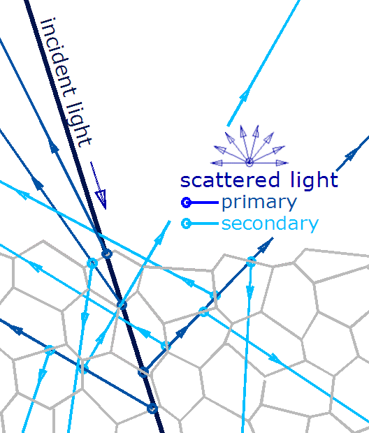
The diffuse equation in the Phong lighting model is the same equation introduced for lighting in the previous chapter: diffuse = L · N or when incorporating light and material values: diffuse = “light color” · “material diffuse” · L · N which is actually a rather realistic model for diffuse light reflections. The specular factor represents direct reflections.

Obviously direct reflections cannot be represented properly without incorporating the complete surroundings. As the only scene objects the Phong lighting model is concerned with are direct light sources its specular term can only be a very crude approximation. The equation is as follows:

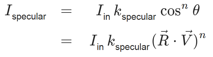
with R being the mirrored vector to the light source (the reflectance vector) and V being the vector to the camera. n represents roughness with 32 being a typical value. A slightly faster and eventually nicer looking equation is the Blinn Phong model for specular reflections:

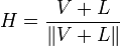
Blinn Phong works with a half vector between the vector to the light and the vector to the camera.

Both models basically calculate a small, direct reflection of the light source. This makes sense because when watching a reflection direct light sources (like for example the sun) are very dominant. Still it’s very far from realistic.

More realistic lighting

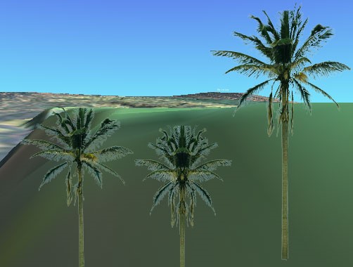
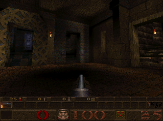
Ambient lighting is an approximation of light bouncing around in the scene. Calculating bouncing light is easy to implement but correct implementations are computationally very expensive and thus not possible in realtime. But ambient lighting does not introduce hard borders in an image, instead it’s all just soft gradients. Bilinear filtering works nicely for soft gradients and as such it is possible to precompute proper ambient lighting and to put it in small textures which are then bilinearly filtered.

Precomputed ambient lighting very much defined the look of early 3D games like Quake and is still widely used today.

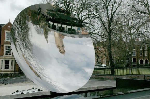
Specular lighting sadly cannot be precomputed as easily. Direct reflections are dependent on the camera position. For some objects in a game it can however make sense to compute the view of the surroundings from the object’s position, encoding the images in a so called cube map. A cube map is a texture which includes six images, each for one axial direction (up, down, left,…). A cube map is indexed using a direction vector – which can be the reflection vector to calculate a nice reflection approximation. Calculating six additional views just for rendering a single object is of course overly expensive and should be reduced to one or two visible objects – like for example the player’s car in a racing game.

Shadows

All those lighting models are just approximations of light bouncing around. What happens during the first bounces is typically more dominant and dynamic in a final picture and thus more resources are spend for early bounces. Direct lighting calculates the very first light bounce. Ambient lighting calculates many bounces and is therefore a candidate for static, low-resolution precalculations. Calculating two bounces produces a very well-known lighting effect: shadows.

Shadows are usually calculated by rendering shadow maps. To create a shadow map the current scene is rendered from the light source’s position. But instead of rendering color values, the depth values are copied to the resulting texture. During regular rendering the vertex shader calculates in addition to the regular positions the positions as seen by the light. In the fragment shader the shadow map is read at the resulting x and y light position and compared to the newly computed light depth positions – a smaller value in the shadow map means that the currently rendered position is further away from the light than the what the light rendered at that x and y positions and is consequently in the shadow.

Shadow maps easily run into precision problems. Reducing precision problems in shadow maps is a current research topic but a widely used method is to use multiple shadow maps for different distances from the camera. Those are called cascaded shadow maps.