Physics
Introduction and Motivation
Physics have been a large and growing part of games for a long time. Starting from the first games like Asteroids, Pong or SpaceWar!, physical properties of objects and their movement have been simulated to make games more believable or enjoyable.
In some cases, this has resulted in game concepts that would otherwise not have been possible. Applications like Bridge Builder (http://www.bridgebuilder.de/) require a physical simulation as it lies at the core of their gameplay to have it.
In some cases, physical simulation can also help with the authoring or creation of the game. Instead of having an artist animate a physical object and its movement, this work can be carried out by a computer.
However, as thousands of physics glitches video on the net show, physical systems are also notoriously hard to program. Once the right conditions are found, almost all systems can be broken in some way or another.
A complete discussion of the principles needed to build production-quality physics code would require much more space than we have available in the course of the lecture. Therefore, we will concentrate on the basic principles.
Examples
- Barrels, Boxes Scenery objects such as barrels or boxes that are part of many industrial or urban environments has become a trope in games. Their ubiquity is partly due to their small complexity. For collision detection, both cylinders (barrels) or boxes can be calculated very efficiently as compared to other convex polyhedra, and therefore are simpler to integrate into games than other objects.
- Ragdolls Ragdolls refer to articulated bodies that are simulated by simulating the body as a chain of bones (see skinning in lecture 7 [[Bumps-and-Animations]]) that have some constraints (they must not be separated - well, in most games that is…, and they should not move beyond the limits that normal human joints have). Previously, ragdolls used to be used only for unconcious or dead characters, as those characters have no movement (animation) of their own accord and are governed completely by external characters. Newer systems have broken up this requirement by mixing forward kinematics (animations) and inverse kinematics as well as ragdolls to create mixtures of ragdolls and animated characters. An example is Euphoria (http://en.wikipedia.org/wiki/Euphoria_(software)), which was used in recent parts of Grand Theft Auto to simulate characters struggling to stand or being bumped into by other characters.
- Soft bodies Few games simulate soft bodies, but support is starting to get better, especially with the movement of calculations of phyics being moved to General-Purpose GPU units (e.g. using CUDA or NVidia PhysX). This allows the simulation of objects such as cloth or hair.
- Fluids, gasses
Motion Physics
The simulation of objects in games often relies on the three laws stipulated by Newton:
-
Every object in a state of uniform motion tends to remain in that state of motion unless an external force is applied to it.
-
The relationship between an object’s mass m, its acceleration a, and the applied force F is F = ma. Acceleration and force are vectors (as indicated by their symbols being displayed in slant bold font); in this law the direction of the force vector is the same as the direction of the acceleration vector.
-
For every action there is an equal and opposite reaction.
Analytical (closed) solutions
As we will see shortly, we can derive differential equations from Newton’s laws and solve them numerically. However, some games use the analytical solution to the physical movmement. An infamous example is gorillas.bas, one of the games included with QBasic. In this game, two gorillas on rooftops are battling it out by throwing explosive bananas at each other, your goal is to hit the other gorilla before he hits your gorilla.
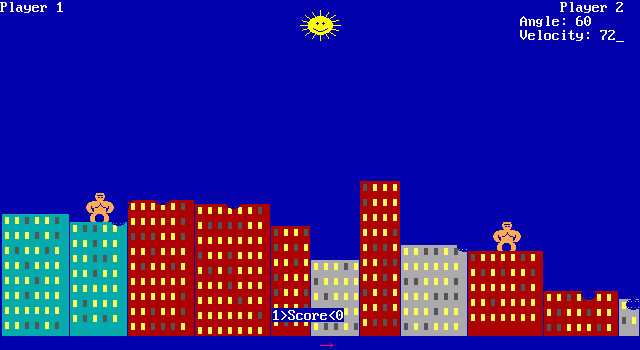
Have a look at the code from the PlotShot function of gorillas.bas:
x# = StartXPos + (InitXVel# * t#) + (.5 * (Wind / 5) * t# ^ 2) y# = StartYPos + ((-1 * (InitYVel# * t#)) + (.5 * gravity# * t# ^ 2)) * (ScrHeight / 350)
This code features the closed solution you probably learned in school for a thrown object under gravity. http://en.wikipedia.org/wiki/Gorillas_(video_game)
Compare the situation to a current 3D game with a physics simulation. We rarely have a situation where we only throw an object. Rather, objects are subject to many forces at the same time. For example, a crate in a game might be influenced by gravity, the force that pushes it out of the ground and the force of the player pushing it away off-center. Finding the analytical solution to such a situation is nearly impossible and would be highly impractical, as it would require new implementations for each possible kind of situation.
Instead, physics engines are usually built upon numerical solvers for the differential equations.
Numerical integration
We first derive the equations for motion of an object from Newton’s second law. This states that F = m * a, or force being equal to mass times acceleration.
We know that a is the change in velocity of an object over time. We can write a = dv/dt to mark this differentiation.
Then, velocity is actually the change in position over time. Therefore, v = dx/dt if x is the positon of our object.
We get a second-order differential equation for F: F = m * dx/dt^2.
Euler integrator
The simplest scheme for integration of the equations is the Euler integrator. This integrator takes two moments in time, which we can for now take to be the time of the previously rendered frame and the current frame. We start with the forces that act on our body and sum up the forces to find one net total force. This is allowed by D’Alambert’s principle, which states that the sum of the forces is equivalent to calculating the effect of each force alone. Note that gravity is often given as an acceleration a = 9.81 m/s^2, and therefore should not be added the same way as a force is added.
From the equations, we know that force and acceleration are related via the mass of the object. We take the current acceleration to be the forces acting on the body divided by the mass of the body.
a = F/m
Using the acceleration, we can estimate the velocity by adding the acceleration to the previous velocity. We use the duration since the last calculation in this calcuation as deltaT:
v_new = v_old + a * deltaT
Finally, we reach the current position of the object by adding the velocity to the position in the previous frame, again, using deltaT:
pos_new = pos_old + v_old * deltaT
To make the whole system behave more realistically (objects have no simulated drag, and will never lose energy), we can add a damping factor. This factor can be a constant in the range of 0 and 1, which we multiply onto our calculations to simulate energy being lost.
v_new = v_old + a * deltaT * dampingFactor
The Euler integrator works relatively well while we have no complicated forces acting on our bodies and especially while we have no collisions.
Integration step
The individual step during one calculation for an object are:
- Calculate the new position by pos_new = pos_old + v_old * deltaT
- Retrieve the sum of forces F from the accumulator and calculate a = F/m
- Calculate the new velocity by v_new = v_old + a * deltaT * dampingFactor
- Clear the accumulator (to allow new forces to be added in the next frame)
Collision detection
As we have noted above in the case of the Euler integrator, collisions are actually where physical simulation gets very interesting.
Collision detection is the task of finding out whether two objects (e.g. a game character and the terrain of the game) are touching or overlapping. In the real world, solid objects could not really “overlap”. They might break or be squished. Due to numerical precision and the impossibility of having an infinitely small time step in the integrator, we will almost never have the case where two objects are touching at exactly one point during collision detection. Instead, the objects will usually overlap. In this case, it is also an important information how much overlap we have. We refer to this as the penetration depth.
Furthermore, we will make use of the collision normal. This normal vector shows us the axis along which the two objects are colliding, and on which we need to separate the objects.
Collision detection is usually a costly undertaking. Especially for complex objects such as meshes with many polygons, it can take a lot of processor time to compute the intersection test. Physics engines a large share of their computational power to find and resolve them.
We provide two easy collision tests here. Collisions between spheres are among the easiest collisions to detect. And planes are often used as the ground plane of a level.
Collision between spheres
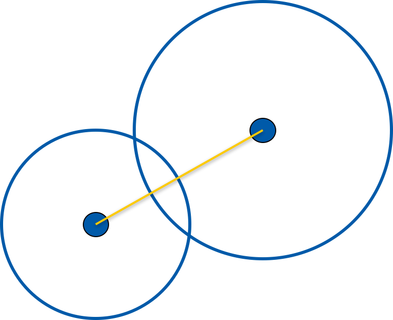
Collision test
We can use the sum of the radii of the spheres to define a minimal distance between the sphere centers. If the sphere centers are closer to each other than this minimal distance, they are colliding.
Collision normal
The collision normal is the vector pointing from one sphere’s center to the other sphere’s center
Penetration depth
In the collision test, we have already calculated the distance between the sphere centers. Similarly, we can compute how much closer they are than the sum of the radii
Collision sphere-plane
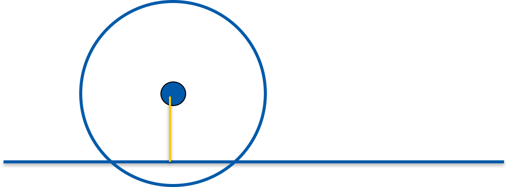
To calculate the collision between a sphere and a plane, we use the Hessian normal form of a plane. This is defined by a normal n and the distance of the plane to the origin, d. We can then use the dot product to map any vertex v onto the normal n. Then, we find the length of this projection and compare it with d. The formula for the distance of a point to a plane is distance = n * v - d
Collision test
We use the distance of the sphere’s center to the plane to find out if they are colliding. If distance < radius, the sphere and the plane are colliding.
Collision normal
The collision normal is the normal n of the plane.
Penetration depth
Use the distance of the sphere and the plane (see calculation above) to calculate how much the sphere penetrates the plane.
Collision resolution
When all collisions have been found, we continue with the resolution of the collisions. We want our objects to move away from each other (separate them) or have them resting on each other if the velocity is slow enough.
To do this, we first calculate the separating velocity. This is the relative velocity of the involved objects mapped onto the collision normal (where one, such as the ground, might be stationary).
To find this velocity, we first map the velocities of the objects onto the collision normal using the dot product. If this velocity indicates that the objects are separating already, we have nothing to do (take care of sign errors which can easily creep in at this point!).
If the objects are moving closer to each other, we have to find a new velocity that they should have after the contact is resolved.
Intuitively, we know that the velocity is opposite to the incoming velocity. This indicates that we should negate the separating velocity and set this to be our desired velocity after collsion resolution.
Second, we know from experience that objects do not bounce forever. In reality, objects loose energy when they collide, or rather, the energy is turned into other forms of energy such as heat or deformation. To simulate this, we can make use of a coefficient of restitution, a value between 0 and 1 which indicates how much velocity should remain after the collision has been resolved. We multiply our desired velocity by this value and get the final desired velocity.
If we apply a delta that changes our current velocity to this desired velocity, we are applying an impulse. This impulse is a momentary change in the velocity of an object and could not happen in reality. Therefore, our object instantaneously changes direction. We calculate this impulse by finding the delta we have to apply to our velocity and just add this delta.
Furthermore, we have to get rid of the penetration. Imagine a ball bouncing. If it penetrated the ground by amount x, and we did not fix the penetration before continuing, it would start it’s bounce from a lower height than if it was sitting on the ground. During the next contact, it might be even further in the ground, and start “hammering” itself into the ground.
Therefore, we move the objects involved in a collision apart from each other after velocities have been adjusted. If one object is immovable such as the ground, our task is clear: We have to move the dynamic object all the way. If two dynamic objects are involved, we should move both of them. A good way to distribute the distance they have to move is by using the masses of the objects and their ratio.
Particle Systems
The equations of motion can be used to simulate particles, infinitisemally small objects. If a system of similar particles is simulated, many visual effects can be achieved, such as gases, fires or explosions. Each particle is usually drawn by placing a small texture in the world at the position of the particle. This is referred to as billboarding.
Emitters
Particle systems use emitters to control the creation of particles. An emitter could be a simple shape such as a sphere or box, or a 3D mesh. Then, particles are spawned in different ways on or in this emitter. They could be randomly created inside the volume of the emitter or on the outside. Usually, the particles’ velocities, masses or other control parameters are also randomized so they appear to be more natural.
Billboarding
When the particles are drawn, the usual technique is to generate a small quad by aliging two triangles in a quadratic shape. Onto this quad, a texture is placed. Usually, to hide the corners of the quad, the texture is drawn using alpha-blending and the texture has alpha=0 at the edges of the quad. This means that particles should be drawn after all solid objects have been drawn, and should be drawn in the correct depth order. However, particle systems can look and feel right without depth sorting, which should only be done if the visual effect that was intended cannot be reached without the depth sorting.
Aligning the billboards to the camera
In many particle systems, the billboards should be visible from all directions in the same way. One way is to rotate them so that when their model matrix is multiplied by the camera’s view matrix, the rotation is cancelled and the billboards face forward in screen space. To do this, we need to multiply them with the camera’s inverse view matrix.
The view matrix is usually the combination of a translation (where the camera is placed) and a rotation (where the camera is looking). We do not care about the translational part of the view matrix, which allows us to just take the 3x3 part of the view matrix that is a rotation matrix. This has the added advantage that the inverse of this matrix is the same as the transpose, which is easier to calculate. With this inverted camera rotation matrix, we can modify the model matrix of the billboard to result in a front-facing billboard under all view angles.
Control parameters
Many control parameters can be defined for particles. One of the most common is the time to live. This time indicates after which duration the particle should be removed from the simulation. This keeps for example a smoke particle system to letting the smoke rise forever. Other control parameters are the change of size or rotation of billboards over time, a tinting color (including alpha) to change the color and alpha of the texture, and many more.