Physics 2

Rigid Bodies

So far, we have not taken care of an important property that separates rigid bodies from particles: they have an orientation and can therefore rotate. This will lead to several additions to the handling of rigid bodies in physical simulations.

Rotation

To add rotation to our rigid bodies, we have to add several properties. The first one is the orientation of the body. Depending on what we use in our engine, we can choose one of the representations we have looked at in previous chapters: Euler angles, rotation matrices or quaternions. Since we will be handling rotation very similar to linear movement and will want to add up rotations, rotation matrices are not well suited to this task, so quaternions or a vector with Euler angles would be more advantageous.

By saving the rotation with our rigid body, we can supply this rotation during rendering as part of the object’s model matrix.

To keep track of changes to the orientation, we will be using the same concepts as we used in linear movement of bodies: the change of rotation over time is the angular velocity. The change in angular velocity over time is the angular acceleration.

Torque

When a force acts on a rigid body, it can turn the object as we can easily find out if we interact with real objects. It is important to note that we can apply a force without inducing a rotation of the body. If we push an object such as a table and do this right in the middle of the table, it will only move linearly, and will not rotate. If we push on one side only, however, it will start to rotate and move linearly at the same time, depending on where exactly we pushed.

This concept is found in physics as torque, which we can think of as the angular component of a force. Whenever we apply a force to an object, the force will be working on the body linearly. This means that we can add it to our (linear) force accumulator. Additionally, we have to compute the amount of torque caused by the force.

A force will have no torque component if it is applied towards the center of mass of the rigid body. This center of mass is where you would balance an object such as a spoon on your finger. It is often identical to the geometrical center of the object, but this is not necessarily so. Think of a box that is made half out of wood and the other half lead - it would not have its center of mass in the center of the box.

In many cases, the center of mass (COM) is not computed by the engine, but the model is supplied by an artist such that the COM lies at the origin in model coordinates. We can also calculate the center of mass, assuming that the mass is distributed uniformly over the object. In this case, the calculation of the center is identical to finding the geometric center.

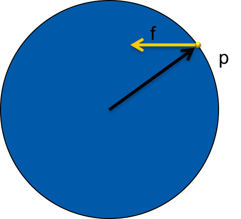
To find the torque component, we need to find the point at which the force was applied to the object. If we call this point p, it is supplied by p - COM, the vector from the center of mass to the point. To find the torque t generated by force f, we use the cross product.

t = (p - COM) x f

This force is added to a torque accumulator just as the forces are. D’Alambert’s principle that allows us to add up forces and continue calculating with the net force extends to torques as well.

Note that in outer space, pushing on an unsuspended object anywhere on the object would also lead to linear movement. On earth, we will usually have friction that keeps the object in place partially, leading to what appears to be pure rotation only.

Mass Moment of Inertia

During the integration step, we now want to update the orientation of the body. To do this, we need to find angular acceleration and velocity. In the linear case, we could use a = F/m, dividing the force accumulator by the mass of the body. In the angular case, we cannot use the mass.

If you think of a lever, it is intuitive that an object resists changes in angular velocity differently according to the point of application of the force that caused the torque. To calculate this correctly, we need a construct that can deal with rotations in a similar way as the mass worked for linear velocity.

This property is referred to as the Mass Moment of Inertia (MOI). The moment of inertia is written as a tensor, a generalized form of a matrix. However, for game physics engines, the mass moments of inertia are usually 3x3 matrices.

To find the MOI, we can look up formulas for simple geometric shapes such as spheres or boxes. The MOI matrix contains on the diagonal the amount of inertia that the object has when it rotates around its principal axes (x, y, and z of the model). The other parts of the matrix encode the way in which the object rotates due to torques when the rotation is around other axes.

If we have a more complex object such as a character represented by a triangle mesh, we can use different approaches. The most exact is to compute a MOI by discretizing the volume of the object and calculating a MOI from this. We can also combine different MOIs of simple shapes to approximate the more complex body. In many cases, since the MOI is not a property that is directly visible, it does not need to be 100 % exact.

To use the MOI, we need to take two things into account:

1. If we have our torques in world coordinates, we need to either map them into object coordinates and then use the MOI, or we need to transform the MOI into world coordinates. If we did not do this, the MOI would not be correctly rotated to follow the shape of the rotated body that we can see on the screen. This would mean that we would not see the movement that we are expecting from reality.
2. We actually need the inverse of the MOI. Exactly as we divided by the mass to find acceleration, we are now using the matrix inverse of the MOI and use this to multiply the torque value.

Friction

Friction is one of the properties that are immediately visible when they are not implemented in a physics engine. If friction is not simulated, we can see that objects will never rotate even when they are sliding across each other.

Friction is a force that is generated when two objects are resting or sliding across each other. In reality, it is created by miniscule irregularities in the surfaces of the objects, where they interlock and result in a force.

Friction is composed of two parts:

• Static friction: This is the friction that keeps objects from sliding across each other if the forces acting on them are not large enough to move them. This is the force that you experience when you start pushing on an object and it won’t move until the force is large enough. It is also the same force that allows mountain climbers to wedge themselves between two walls and “walk” up - static friction keeps their feet on the side of the rock.
• Dynamic friction: Once the static friction has been overcome, the object(s) will start to move. The friction acting on them is dynamic friction.

The amount of friction is stated by Coulomb’s law of friction, which states that the amount of friction is less than or equal to the amount of normal force multiplied by a friction coefficient. Normal force is the amount of force that acts in the direction of the collision normal. The coefficient depends on the materials that are in contact: Metal on ice has a different coefficient than cloth on wood.

In practice, we often choose the maximal value to get rid of the inequality.

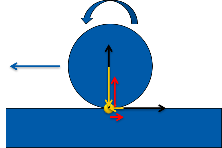
The direction of the friction force is opposite to the velocity of the object, in the plane across which it is sliding.

Collision basis

To handle friction, it is very advantageous to calculate a collision basis. This basis is a set of vectors that make up an orthonormal basis of a coordinate system. In this coordinate system, the first vector x is the collision normal. The other two vectors are perpendicular to the first one and define the plane across which the object is sliding. This is an approximation: Since we are only handling one point of contact, we can imagine that we are sliding across a plane, even if the object is curved.

When handling velocities to handle contacts, we will be handling the x-component of the collision velocity the same way as we did before. To do this, we need to take into account the rotation as well now, which can change the velocity with which the point of collision collides with the other object. Imagine a rod being held into a the rotor blade of a ventilator: The blade has no linear movement, but the impact of the blade on the rod has velocity due to the rotation of the blade.

This means that we need to map the velocity into the collision basis. This will tell us how much the objects are moving towards each other and at which speed the objects are sliding across each other.

In the collision basis, we can then find the amount of the velocity in the plane. We can estimate the impulse that friction generates by a coefficient. This impulse takes velocity away from the velocity of the object, i.e. it is opposite to the object’s movement along the plane.

This way, we are handling friction in the same way as we have been treating collisions: We changed the velocity of the object instantly by applying impulses.

We will not be going further into the details of friction computation here.

Collision detection refined

Collision detection is usually a costly undertaking. Especially for complex objects such as meshes with many polygons, it can take a lot of processor time to compute the intersection test.

A common scheme to reduce this load lies in finding ways in which we can reduce the workload by not carrying out superfluous calculations. If we have a way of showing that two objects can under no circumstances intersect with a cheap method, we can skip the costly detailed method for collision detection for these objects.

The easiest way to implement such a scheme is to create simple bounding objects and carry out the collision detection with these objects. This step of ruling out possible collisions is referred to as the broad phase of collision detection. We don’t care about the details of any collisions but about a broad overview of the collisions that are realistic to be actually happening.

Bounding objects

Usually, the broad phase makes use of bounding objects that can be efficiently tested for collision. The most simple and computationally cheapest collision test is between two spheres, which is why they are a good candidate for bounding objects.

As long as the sphere completely contains the objects to be tested, we can test the objects for possible collisions by checking the bounding spheres. If the spheres do not collide, the objects cannot contain. If, however, the spheres collide, the objects might or might not collide. To determine this, we have to test the objects in the narrow phase again.

We want to have bounding objects that approximate the objects as well as possible. In general, we want a convex shape for the bounding object. Non-convex objects are much more costly to test for collision. As you can see from the spheres, they only approximate objects well that are essentially spherical. Long, narrow objects waste a lot of space - the more empty space in the bounding body, the less reliable the test will become, as the actual objects might still be far away when the bounding bodies already touch.

The most common bounding objects are:

• Spheres
• AABB’s (Axis-aligned bounding boxes) are boxes whose planes are aligned with the global x, y and z axes. This means that the collision test for these boxes is relatively cheap as we do not have to account for different angles of the bounding boxes, but they can fit badly to rotated objects.
• OBB (Oriented bounding-boxes) are boxes that are rotated to follow the shape of the object. These boxes approximate the shape of many rotated objects well and are therefore better in this respect than AABB’s, but are most costly to evaluate under collision.
• Capsule: A capsule is a mixture between a sphere and a cylinder. This kind if shape is still easy to compute, and is often used for approximating characters.
• Convex collision shapes: In same cases it can make sense to build a convex shape in a graphics program that approximates a certain shape very well. This bounding shape would usually be much less detailed than the contained object and therefore easier to compute for collisions. Note that in some cases also the narrow collision is handled by a simplified object. For example, a character can, in many cases, be approximated by a capsule collider.

Bounding Volume Hierarchies

Even if we have bounding objects in the broad collision detection phase, we have to check all pairs of bounding objects in the broad phase in a naive implementation. Every addition of an object adds further collision tests. To minimize this cost, we want a sense of locality, meaning that we only test those objects that are relatively close. One possible way to implement this is by implementing bounding volume hierarchies. We apply the same idea to bounding volumes that we applied to the original objects, i.e. we create bounding objects for bounding objects. This results in a hierarchy with larger bounding objects in the top of the tree and smaller ones further down. When testing an object for collision, we can exclude a much larger number of collisions if we find a large bounding object that tells us that the collision is not possible for all sub-objects.

Spatial data structures

A similar idea is followed by spatial data structures. These data structures help us organize the objects in the world by location. The easiest data structure is a regular grid. For each object, we save in which grid field(s) it currently is. We can then use this information for example to find out which pairs of objects might collide (those occupying the same grid fields).

More advanced data structures in 3D are Octtrees, kd-trees and Binary Space Partitioning Trees.

• Grid A grid can be defined by a point where it starts and the regular grid cell size. During lookup, we have to find which cells our object lies, and we can look up which other objects are in the same cells. During saving of the grid, we need to take care that we save references to each object in all relevant grid cell.
• Octree(3D), Quadtree(2D) The idea of these two structures is to start with a rectangular volume. Then, this space can be narrowed down by subdividing it into 4 (quadtree) or 8 (octree) volumes. This is continued until a minimal number of objects per grid cell is found.
• KD-Tree The KD-Tree is the generalization of an octree/quadtree. The idea is to start again with a rectangular volume. Then, during each step, a new plane is chosen that intersects one old grid cell. This is done alternatingly for each axis. In 2D, this would be alternating between horizontal and vertical lines as separators. This way, the kd-tree can better handle clusters. An octree might have to be subdivided often if a cluster is badly placed. In a kd-tree, the plane can be chosen to intersect the cluster immediately and split it in half.
• BSP-Tree (Binary Space Partition) The BSP can be thought of as a generalization of the kd-tree. Instead of having axis-aligned planes that separate space, we choose planes at randomly, which subdivide space into half. This can be used to even better work with the shapes that are found.

Narrow phase

Once the broad phase has finished, we consider only those objects that might still be colliding. In general, the tests used here will be more computationally expensive than those in the broad phase. Still, we want them to be as fast as possible to be usable in realtime games.

Most of the algorithms for collision detection assume that the objects are convex. This assumption leads to the advantage that we can not have the situation where one object fits into a “nook” in the other object.

While it is possible to create games only using convex polyhedra, it is often unfeasible. For example, human characters are non-convex. In such cases, the object is often broken down into convex parts. For example, the character can be approximated by either a capsule, or, if more detail is required for collisions, by a set of boxes and capsules for the torso, head and limbs. This process if often performed by artists by hand to realize a performant solution, but algorithms exist which can carry out this tasks (creating convex sub-meshes from non-convex meshes) automatically.

Separating Axes Test

One possible way of deriving a collision test lies in the Separating Axes Test.

The idea is that if two objects are not overlapping, there must be a plane we can draw between them so that object 1 is completely on one side and object 2 completely on the other side. This also means that there must be an axis, perpendicular to this plane, that separates the two objects. More exact, it indicates that there is an axis such that if we project the objects on the axis, the line segments that we project on do not overlap.

This would not really limit us very much, since we have a possibly infinite set of axes that could be candidates. However, it can be shown that for polygonal objects, only the relevant features have to be tested for separation.

In the slides you can find the example of a sphere-triangle intersection test based on the SAT. The relevant features of the triangle are the face, the edges (x3) and the vertices (3). The sphere has no clear features, however, we can construct one for each test: The closest point on the sphere to the feature defines an axis to test for.

Using the SAT, we have to test all possible axes for separation. Once we have found a separating axis, the test is finished. However, if the objects are intersecting, we can only know this for sure when all candidate axes have been identified.

Note that this test will not tell us where the objects collided or what the collision normal was. The computations of the test will often be helpful in finding this information, but the separating axes test can only give us the answer of whether two objects are intersecting or not.

Soft body physics, Fluids

Games have started to use soft body physics or to simulate gases. These two ideas are handled in similar ways to the numerical solution we find for the equations of motion. For soft bodies, often, the finite elements method (FEM) is used, where the body is split up into small volumes for which stress and strain are simulated as forces. Fluids work similarly, they are represented as vector fields that indicate where fluid or gas particles are travelling in the fluid.

Using the spring or rod constraints mentioned above, cloth can be simulated. In this case, the cloth mesh is controlled by a grid of particles which are connected to their neighbors by constraints.

Constraints

Except for specifying and keeping track of objects not intersecting, we can add other constraints to our objects. We can differentiate between stiff constraints and flexible constraints. The first category would be a metal rod that connects two objects: They are kept at an exact length apart from each other. The second constraint is realized by simulating a spring.

If a spring is pulled or compressed out of its rest length, it will generate a force on the bodies that are connected to it. Hooke’s law formulates that the resulting force is equivalent to the rest length multiplied by the coefficient referred to as the stiffness factor.

During the simulation, we also need to keep track of the constraints and ensure that the objects are correctly based on their constraints.

Note that adding very stiff springs or constraints that are similar in nature, the whole system of equations will become “stiff”, meaning that our integrator has to use ever smaller time steps to get a good solution. Otherwise, the system will become unstable and might “explode”, leading to a situation where ever more energy is created and objects fly apart from each other.

Constraint-based solvers

In our physics engine, we have used an approach referred to as sequential impulses. This approach means that we handle one collision after the other and we use the results of previous collision handling steps in the current computation. This means that we have several problems, for example, stacks of objects can easily become unstable and the order in which we resolve collisions makes a difference.

On the other hand, constraint-based solvers use a different method to solve all collisions and constraints at the same time. These systems derive a matrix composed of equations that capture the constraints that are enforced. Collisions are inequality constraints: The objects should either touch or be separated. Rods between objects are equality constraints: They are formulated as constraints that enforce that the difference in position equals zero.

The resulting equation system is of a form that makes it a Linear Complementarity Problem (LCP) for which efficient algorithms for solving exist.

More physics engine concepts

Time steps

Time steps in physics engines come in two varieties: fixed and adaptive. In fixed time step systems, we have one step size that we always advance time in. After the time has been advanced, we handle collisions at that time.

As we have seen, the moments where no collisions happen do not matter very much in the physics engine. The important moments are those when collisions happen. Therefore, some physics engines step through a time step and set the time to the moment when collisions happen. This needs a collision detection that can detect collisions that are about to happen or that happened between two points in time. This kind of collision detection is referred to as continuous collision detection.

Different numerical solvers

The Euler integrator is neither very robust or exact. Numerical analysis shows that it is not very resistant to errors. For our purposes, it has sufficed so far. We can see that it is inexact if we try to use it to integrate a very complex curve. Since we use only the gradient at the time where we compute our time step, it has a hard time following the curve, especially if the time step is too large. Other integration schemes are more resistant and have less errors.

Two often used examples from game physics are the Runge-Kutta method of 4th order (RK4) and the velocity-less Verlet integration.

RK4

The Runge-Kutta-integrator’s difference to the explicit Euler integrator is the fact that the RK4 scheme uses four gradients of the function it integrates as compared to only one for the Euler integrator.

Velocity-less Verlet

Velocity-less Verlet integration is another scheme for integrating the equations of motion that uses does not explicitly use velocity. Instead, it works on the difference between the last time step’s position and the current position. This makes it well suited for physics as we have been simulating them, where we move objects to get rid of interpenetrating, since we do not have to calculate the impulse that is necessary for this.